Errata for the Paper “Reducing Artifacts of Focused Sources in Wave Field Synthesis”, 129th AES Conv., San Francisco.

This post contains an errata for the paper:

Wierstorf, Geier, Spors: Reducing Artifacts of Focused Sources in Wave Field Synthesis, 129th AES Conv., San Francisco.

The scale of the y-axis in Fig. 4 of the paper is wrong! The value for t (ms) should be -5 and not -0.5.

Posted in Papers | Leave a comment

Audio Examples for the Paper “Reducing Artifacts of Focused Sources in Wave Field Synthesis”, 129th AES Conv., San Francisco.

This post contains supplementary audio examples for the paper:

Wierstorf, Geier, Spors: Reducing Artifacts of Focused Sources in Wave Field Synthesis, 129th AES Conv., San Francisco.

Please use headphones to appreciate the spatial information!

The provided files are named using the following scheme:

<array length>_<radius>_<angle>_<input sound>.wav

Array lengths are 10 m, 4 m, 1.8 m, 0.75 m, 0.3 m; the radius (= distance from the focused source to the listener position) is 1 m and 4 m, respectively. The focused source is always located one meter in front of and in the middle of the loudspeaker array. The angle is 0, 30 or 60 degrees. The input sound is either castanets or female speech.

The geometry of the experiment is shown in the following figure.

Sketch of the geometry used in the experiment

In addition, there are also 2 reference stimuli, ref_1m_0_speech.wav and ref_1m_0_castanets.wav using plain HRTFs for the frontal direction.

You can download a ZIP-file with the speech examples and a ZIP-file with the castanets examples.

More detailed information can be found in the paper and in the slides.

Errata: The scale of the y-axis in Fig. 4 of the paper is wrong! The value for t (ms) should be -5 and not -0.5.

Posted in Papers | Tagged , , | 1 Comment

New papers published

We have recently published some papers:

  • at the 40th International AES Conference in Tokyo
  • at the ITG-Fachtagung Sprachkommunikation in Bochum, Germany
  • in the IEEE Transactions on Audio, Speech and Language Processing
  • in the EURASIP Journal on Advances in Signal Processing

You can find the references and download the papers in/at my publications list.

Posted in Anouncements, Papers | Leave a comment

Presentation about Using the SoundScape Renderer for Psychoacoustic Experiments

I just held a presentation called “Conducting Psychoacoustic Experiments with the SoundScape Renderer” where it was shown how to use the SSR for subjective tests involving spatial audio.

The slides can be downloaded here.

The corresponding paper is available here.

If you got interested, you can download the SSR here: http://tu-berlin.de/?id=ssr

Posted in Papers | Tagged , | Leave a comment

Audio examples for paper “Ahrens, Wierstorf, Spors: Comparison of Higher Order Ambisonics And Wave Field Synthesis With Respect to Spatial Discretization Artifacts in Time Domain. 40th AES Conference”

This post provides supplementary audio examples for the paper

Jens Ahrens, Hagen Wierstorf, and Sascha Spors: Comparison of Higher Order Ambisonics And Wave Field Synthesis With Respect to Spatial Discretization Artifacts in Time Domain. 40th Conference of the AES, Tokyo, Japan, October 8-10, 2010 [ pdf ]

NOTE THAT THESE EXAMPLES ARE INTENDED FOR HEADPHONE REPRODUCTION!!! The examples were prepared from BRIR measurements of a real loudspeakers system. They contain the signals for 0° orientation of the listener (i.e. straight forward). The setup is explained in detail in Sec. 3 of this paper.

Download zipped files for speech.

Download zipped files for castanets.

Download zipped files for pink noise.

In the data you find the raw input signals, plus HOA and WFS examples. The file names are composed of the input signal, the method, and the listening position.

Posted in Papers | Tagged , , | Leave a comment

Using an eye tracker for acoustic localization experiments

We have evaluated the use and accuracy of using gaze captured by a head-mounted eye tracker in acoustic source localization experiments. The results can be found in a recent paper presented at the 38th International Conference on Sound Quality Evaluation of the Audio Engineering Society. The following video shows a snapshot of the conducted experiments as seen from the helmet camera of the eye tracker

Seven loudspeakers at known positions are located behind the acoustically transparent gray curtain. The stimulus is played from a random loudspeaker and the subject is asked to fixate the perceived position of the stimuli. The gaze is tracked by the eye-tracker and shown as overlay in the video. The subjects were additionally asked to point to the perceived source position using a laser pointer. The pointer is also visible in the video. The details of the experiment can be found in the paper.

Posted in Papers | Tagged , | Leave a comment

Facebook Group

We have created a facebook group “Spatial Audio Research” for general discussions, announcements and sharing links:

Posted in Anouncements | Tagged | Leave a comment

Updating multiple SVN working copies at once.

This is not really audio related, but maybe someone is interested anyway …

We use Subversion (SVN) for several different things — software, papers, scripts — and one of the most common tasks is to update working copies all over the place. This can be quite annoying if you are working on many SVN repositories.

To make this repetitive task a little easier, the following scripts can be used.

Therefore, create a new directory and put all your working copies in subdirectories and use one of the following scripts to do the rest of the work.

Windows

I suppose you have TortoiseSVN installed — if not, install it.

Put the following in a file with the extension .bat, place it in the directory with your working copies and double-click on it.

@echo off
FOR /D %%A IN (*) DO START TortoiseProc.exe /command:update /path:%%A /closeonend:0

(The basic idea is stolen from here.)

Linux/Unix/…

Put the following code in in a file, make it executable and put it in the directory with the working copies (or somewhere in your path, e.g. in $HOME/bin/). Then start the script.

#!/bin/bash

# Shell script that runs "svn update" in each subdirectory.
# If arguments are given, they are used instead of "update".
# The script also works if a directory name contains spaces.

COMMAND=svn
# if no options are specified on the command line, this is used:
OPTIONS=update

LOGFILE=error.log

if [ $# -gt 0 ]
then
  OPTIONS="$@"
fi

for DIR in */
do
  echo "============> entering "$DIR""
  (cd "$DIR" && $COMMAND $OPTIONS) 2> >(tee -a $LOGFILE >&2)
  echo "============> leaving  "$DIR""
  echo
done

# if error-log is empty, remove it
if [ $(wc -l < $LOGFILE) -eq 0 ]
then
  rm -f $LOGFILE
fi
Posted in Uncategorized | Tagged | 1 Comment

Auditory Modelling Toolbox (AMT) 0.2 released

A new version of the growing Auditory Modelling Toolbox has been released. The main new feature is a binaural model after Lindemann (1986a) that uses a running cross-correlation with inhibition to predict the perceived lateralization of an auditory event. The output of the model depends on the auditory filters and on the time (see figure below).

To install it, you can download it from Sourceforge. You also have to install the Linear Time/frequency Toolbox. Then in Matlab or Octave just go to the directories of the toolboxes and run:

>> ltfatstart
>> amtstart

After this you are able to use the Lindemann model, see help lindemann for an introduction. To produce the figure below, you can run:

>> demo_lindemann;

Another very nice feature is the function exp_lindemann1986a that is able to reproduce the figures of the Lindemann paper. For example to reproduce figure 6 of the paper, just type exp_lindemann('fig6'). The model is under further development and will include in the next release a version of the method proposed by Gaik (1993) to identify natural combinations of ITDs and ILDs. Further a version of the Breebaart model will also be included in one of the next releases.

Binaural activation map

Posted in MATLAB | Tagged | 1 Comment

An introduction to Gnuplot

For all of you who are looking for an alternative to plotting with Matlab or a tool to create very nice looking plots, Gnuplot is waiting for you.

Since the early days of my studies I’ve been using Gnuplot and just started the Gnuplotting Blog to share some nice solutions and possibilities of Gnuplot with you. There you will find also an short introduction how to use it.

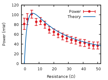
To give you a short idea of how Gnuplot works in the following you see a short Gnuplot script for plotting data and functions and the resulting figure. The data file being used ships with Gnuplot.

Battery data

 
#!/usr/bin/gnuplot
# Plotting data about battery power (see battery.dat)

reset

# wxt
set terminal wxt size 350,262 enhanced font 'Verdana,10' persist

# color definitions
set border linewidth 1.5
set style line 1 lc rgb '#0060ad' lt 1 lw 2 # --- blue
set style line 2 lc rgb '#dd181f' lt 1 lw 2 pt 7 # --- red

set key at 50,112 
set xlabel 'Resitance (Ω)'
set ylabel 'Power (mW)'
set tics scale 0.75

# Therotecial curve
P(x) = 1.53**2 * x/(5.67+x)**2 * 1000

plot [-2:52][0:120] 'battery.dat' u 1🙁$2*1000):($4*1000) 
                        t 'Power' w yerrorbars ls 2, 
                    P(x) t 'Theory' w lines ls 1
Posted in Pictures | Tagged , | Leave a comment